Exercise 3 - Denoising using deep learning method (Noise2Void)
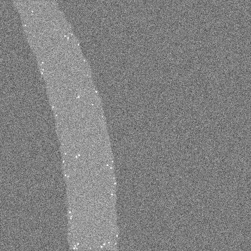
Spinning disk confocal image of FISH in C. elegans (image courtesy of ABRF/LMRG Image Analysis Study).
Open the above Z-stack in Fiji and run the command:
Plugins › CSBDeep › N2V › N2V train + predict
You will be presented with a
N2V train + predictwindow. Choose the following options and click OK.- Axes of prediction input: XYZ
- Number of epochs: 10
- Number of steps per epoch: 10
- Batch size per step: 64
- Patch shape: 64
- Neighborhood readius: 5
A window showing the progress of different steps (Preparation, Training and Prediction) will open. As the training progresses, training loss (red) and validation loss (blue) curves are displayed in the window (see below). If training goes well, then both the red and blue curves will decrease with more cycles (epochs) of training and stabilize around a minimum loss value (~ 1.0 in the image below). Training loss goes down from the beginning but Validation loss (blue curve) usually goes up in the beginning and then comes down and approaches the red curve.
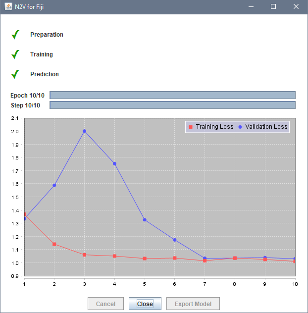
Training deep learning model If by the end of the training, red and blue curves do not stabilize to a minimum loss value, then increase the number of epochs to 20 or 30 and then run the command
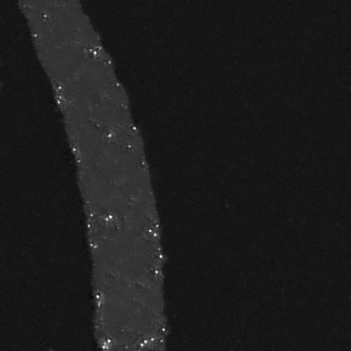
N2V train + predictagain.After program finishes, it generates a denoised Z-stack from the trained model. You might need to run
Image › Adjust › Brightness/Contrast...and hitResetto adjust the display of the denoised image.The Deep Learning model you just trained could be saved as a .ZIP file (to be used for prediction in the future) by clicking on the
File actions > Save to...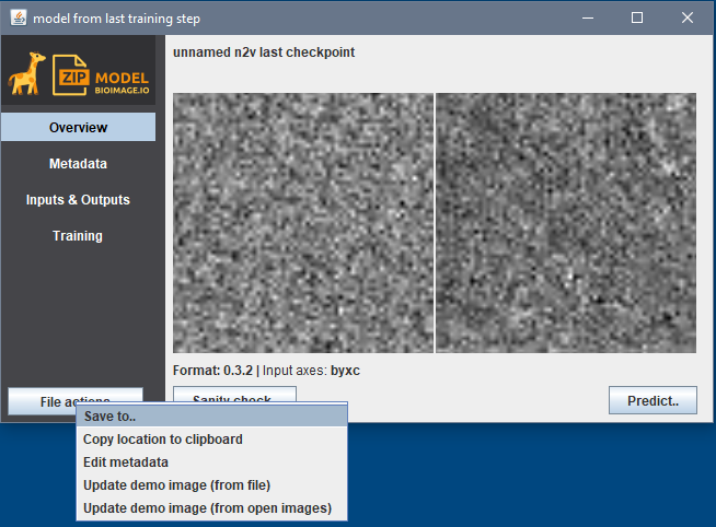
Saving deep learning model Trained model could also be applied immediately on a single noisy image or a folder full of noisy images by using
Predict > Single image or stackorPredict > Folder of images of stacks, respectively.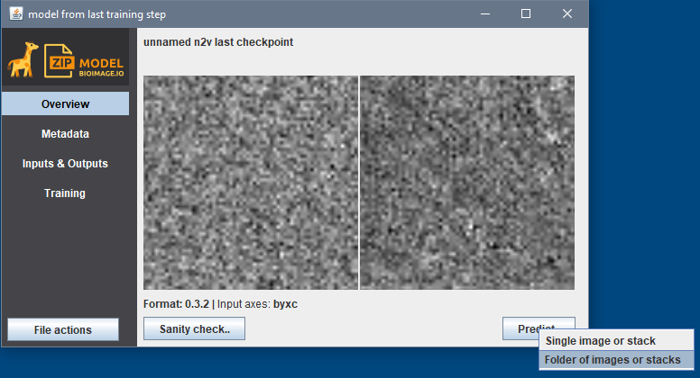
Applying deep learning model